Singular Value Decomposition (SVD) is a linear algebra algorithm that decomposes almost any matrix of numbers into 3 matrices, that when multiplied together will recreate the original matrix. There are several of these matrix decomposition techniques, useful for different purposes.
Before we delve into the uses of SVD, we will take a short detour. The
rank of a matrix is the number of linearly separable rows (or columns) in the matrix, which means that:
if (row[i] + x) * y + z = row[j]
then rows i and j are not linearly separable
Computing the rank is done by mutating the matrix into
row echelon form, which substitutes a row of zeros for all of the rows which are considered "duplicates" under linear separability. Here is a tutorial on row echelon form:
https://stattrek.com/matrix-algebra/echelon-transform.aspx#MatrixA
This matrix has a rank of 1 because it is possible to generate any 3 of the rows from the fourth row with the above formula, and to generate the remaining columns:
[1,1,1,1]
[2,2,2,2]
[3,3,3,3]
[4,4,4,4]
This is called
linear separability. Rank gives a primitive measurement for the amount of correlation between rows or columns. SVD is more nuanced. It implements linear separability as a continuous measurement whereas rank is only a discrete measurement. Separability is scored by Euclidean distance, and SVD creates a relative ranking of how close each row is to all other rows, and how close each column is to every other column. This ranking gives a couple of useful measurements about the matrix data:
- It gives a more nuanced measurement of separability than just the rank. It gives a vector of numbers which give the relative amount of separability across multiple columns.
- By ranking the distances among rows & columns, it gives a scoring of centrality, or "normal vs outlier".
This matrix has a rank of 2 because while it is not possible to generate matching rows or columns, they are close:
[1,2,3,4]
[2,3,4,5]
[3,4,5,6]
[4,5,6,7]
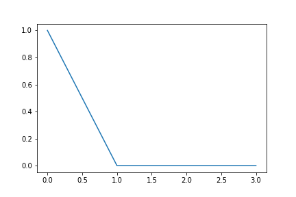
SVD generates a list of numbers called the "singular values" of a matrix. Here are the singular values for the above 2 matrices:
[1.00000000e+00 8.59975057e-17 2.52825014e-47 3.94185361e-79]
[9.98565020e-01 5.35527830e-02 1.96745978e-17 9.98144122e-18]
Let's chart these singular value vectors (linear scale):


These charts tell us that the first matrix has a rank of 1. The second matrix has a rank above one, but does not have two full rows of uniqueness. This chart is a measurement of the correlation between rows and correlation between columns. The singular values of a matrix are a good first look at the amount of "information" or "signal" or "entropy". "Quantity of signal" is a fairly slippery concept with mathematical definitions that border on the metaphysical, but the singular values are a useful (though simplistic) measurement of the amount of information contained in a matrix.
Based on the term "entropy" in the previous paragraph, let's try filling a larger matrix with random numbers. This is the measurement of a 20x50 random matrix, with a chart in log scaled on the Y axis:
Rank = 20
Singular values:
[0.35032972 0.322733   0.30419963 0.29269556 0.28137789 0.26201005
 0.25742231 0.23075557 0.21945011 0.21763414 0.20245292 0.1976021
 0.175207   0.16692658 0.14884194 0.14208821 0.13474842 0.12291441
 0.10004981 0.08849001]


The graph should be a straight line but is not, due mainly to the fact "random numbers" are very hard to come by. This matrix has rank of 20- you cannot multiply & add any row and get another row. In fact, all rows are equidistant under Euclidean distance. Let's do something sneaky: we're going multiply it by itself to get a 50x50 matrix of random numbers. Here's are the measurements (again, a log-Y chart):


Rank = 20
[1.14271040e+02 9.69770480e+01 8.61587896e+01 7.97653909e+01
 7.37160653e+01 6.39172571e+01 6.16984957e+01 4.95777248e+01
 4.48387835e+01 4.40997633e+01 3.81619300e+01 3.63550994e+01
 2.85815085e+01 2.59437792e+01 2.06268491e+01 1.87974231e+01
 1.69055603e+01 1.40665565e+01 9.31997487e+00 7.29072452e+00
 1.50274491e-14 1.29473245e-14 1.24897761e-14 1.11334989e-14
 1.03937520e-14 9.90176181e-15 9.17746567e-15 8.94074462e-15
 8.58805508e-15 7.94287894e-15 6.90962668e-15 6.72135898e-15
 6.02639348e-15 5.66356533e-15 5.16429606e-15 4.84762468e-15
 4.47711092e-15 4.37266408e-15 4.27780206e-15 3.43884568e-15
 3.21440817e-15 2.83815151e-15 2.61710432e-15 2.34685343e-15
 2.24348424e-15 1.32915906e-15 9.12392110e-16 5.65320744e-16
 2.64346262e-16 1.11941235e-16]


Huh? Why is the rank still 20? And what's going on with that chart? When we multiplied the matrix by itself, we did not add any information/signal/entropy to the matrix! Therefore it still has the same amount of separability. It's as if we weighed a balloon, filled it with weightless air, then weighed it again.
In this post, we discussed SVD and the measurement of information in a matrix; this trick of multiplying a random matrix by itself to blow it up was what helped me understand SVD ten years ago. (Thanks to Ted Dunning on the Mahout mailing list.)
I've fast-forwarded like mad through days of linear algebra lecture, in order to give intuitive understanding about matrix analysis. We'll be using SVD in a few ways in this series on my explorations in Neural Networks. See this page for a good explanation of SVD and a cool example of how it can be used to clean up photographs. :
Source code for the above charts & values available at: